TurboFan Engine Degredation Simulation

To put it simply, a turbofan is a jet engine with a fan attached to the front, that acts as a propeller and compression fan to produce more thrust with less energy. The health index of a turbofan is reliant on how far the engine is operating from operating limits like the Exhaust Gas Temperature (EGT) and amount of stalling in the Fan and in the High and Low Pressure Compressors (HPC and LPC respectively).

In this simulation, the fault in the High Pressure Compressor (or HPC) grows in magnitude until system failure. The fault in this case is an HPC compressor stall. A compressor stall occurs when there is an imbalance between the airflow supply and the airflow demand. This creates a pressure ratio that isn't compatible with the engine's revolutions per minute. This in turn makes the air through the compressor slow down. (https://www.skybrary.aero/index.php/Compressor_Stall)

This dataset contains the operational settings and sensor measurements for a simulated turbofan engine going through degredation. It was made due to the lack of run-to-failure data needed for prognostics, which is the reduction of remaining useful component life. Below is a photo from the Damage Propagation Modeling for Aircraft Engine Run-to-Failure Simulation paper about this simulation.

Remaining Useful Life Prediction

Remaining Useful Life (RUL) prediction can be highly useful in maintenence of machines. RUL is useful because it allows us to know when a machine will fail to improve cost savings, and safety. Additionally, it gives decision-makers insight on how they may need to change operational characteristics, such as load, to prolong the life of the machine.

Today, we will be using data from NASA's Turbofan Engine Degradation Simulation to build a model that predicts how many cycles are left in the jet engines life before failure. The general workflow will be:

1. use the Machine Data Hub command line package to download the data
2. process and clean the data
3. do some dimensionality reduction
4. make predictive models
5. assess model accuracy and performance

Using MDH Command Line to Get Data

First, we'll install the Machine Data Hub package

• type pip install mdh into your terminal

Then, we need to get our dataset. Let's find what ID our dataset has in order to download it. We want to use NASA's Turbofan Engine Degradation Simulation Dataset.

• type mdh list to view the datasets and their ID's

We can see the dataset we want has an ID of 9. It also tell us that there are 2 available files. Now we can download the data (make sure you're in a directory where you want the data files to be)

• type mdh download 9 1 to download the first file of the 9th dataset

import pandas as pd
import numpy as np
import random

Understanding the Data

The readme.txt file gives us some context about the data.

• In the training set, the fault grows in magnitude until system failure.
• In the test set, the time series ends some time prior to system failure.
• Also provided a vector of true Remaining Useful Life (RUL) values for the test data.

GOAL: Predict the number of remaining operational cycles before failure in the test set, i.e., the number of operational cycles after the last cycle that the engine will continue to operate.

When building machine learning models, it is best practice that you do not touch the test data until the very end, when you have chosen the "best" model. We will not use the test set until we have chosen a model that we decide is "best" based on metrics we get to choose, that can be found by splitting the training data into training and validation sets.

Training Data

Now we'll read in the simulation data. In this training set, the fault in the High Pressure Compressor (or HPC) grows in magnitude until system failure, also known as run-to-failure data.

You can see that there is simulation data run on many different units with different sets of operational settings and sensor measurements. As we use this data, we want to make sure we can make predictions for each unit, so we need to keep each unit's data together.

train = pd.read_csv('CMAPSSData/train_FD001.txt', sep=" ", header=None)
train.columns = ['unit', 'cycle', 'op1', 'op2','op3','sm1','sm2','sm3','sm4','sm5','sm6','sm7','sm8','sm9','sm10','sm11','sm12','sm13','sm14','sm15','sm16','sm17','sm18','sm19','sm20','sm21','sm22','sm23']
train = train.iloc[:, :26]
units = train['unit']
train.head()

Remaining useful life for each unit

Next, lets read in the file with values of remaining useful life, or RUL, (our target variable) for each unit in test data. We will just look at the first simulation, FD001. In this dataset, RUL is given to us in cycles, which are integers.

RUL is the target data in this case because it is the variable we want to predict. We want to be able to take input data about the engine and output how many remaining cycles we think the engine has.

RUL = pd.read_csv('CMAPSSData/RUL_FD001.txt', header=None)
RUL.columns = ['RUL']
RUL.head()

Test Data

Last, we'll get the test set. In the test set, the time series ends some time prior to system failure.

test = pd.read_csv('CMAPSSData/test_FD001.txt', sep=" ", header=None)
cols = pd.DataFrame(test.columns)
test = test.iloc[:, :26]
test.columns = ['unit', 'cycle', 'op1', 'op2','op3','sm1','sm2','sm3','sm4','sm5','sm6','sm7','sm8','sm9','sm10','sm11','sm12','sm13','sm14','sm15','sm16','sm17','sm18','sm19','sm20','sm21']
test.head()

Data Processing

Looking at range of life cycles each unit ran

Looking at these values will give us a general idea of the cycles the jet engines ran.

max_life = max(train.groupby("unit")["cycle"].max())
min_life = min(train.groupby("unit")["cycle"].max())
mean_life = np.mean(train.groupby("unit")["cycle"].max())
max_life,min_life,mean_life

(362, 128, 206.31)

Setting up X and y in training and testing data

Setting up Remaining Useful Life variable (y)

The data gives us measurements from each cycle counting up, but we want the remaining useful life, or the cycles left before failure. In order to set up the data to have remaining cycles left, we will reverse the cycles column so that instead of counting up, it's counting down until failure. This will ultimately be our target y variable.

## reversing remaining useful life column so that it counts down until failure
grp = train["cycle"].groupby(train["unit"])
rul_lst = [j for i in train["unit"].unique() for j in np.array(grp.get_group(i)[::-1])] # can be used as y or target for training

Setting up sensor measurements (X)

Since we are predicting remaining useful life, we don't want that column in our X, or input data, so we remove it.

# getting all columns except target RUL column as X
train_x = train.drop("cycle", axis=1)
test_x = test.drop("cycle", axis=1)

Applying Principal Component Analysis

We are applying Principal Component Analysis (PCA) in order to avoid overfitting due to the large number of features in the dataset. PCA reduces the dimensionality of the data by using the given features and linearly transforming them to new features that capture the same amount of variance as all of the original features. Here, we are setting PCA to choose the # of features that explain 95% of the variance in the data.

More info on how PCA works: https://towardsdatascience.com/how-exactly-does-pca-work-5c342c3077fe

from sklearn.decomposition import PCA
from sklearn.preprocessing import MinMaxScaler
from sklearn.preprocessing import PowerTransformer
from sklearn.model_selection import train_test_split, cross_val_score

Fitting PCA and transforming train and test sets

• First, we are setting the "unit" column to be the index of the dataframe for the train and test sets. This is because "unit" is not a feature that will be used to make predictions, so we don't want it to be used in PCA either.
• Next, we scale the data. We fit the scaler on the training set, and transform both training and testing sets with the same scaler.
• Next, we do PCA on the data. We fit the PCA on the training set, and transform both training and testing sets with the same PCA.
• Last, we save the results of PCA as dataframes.

# fitting PCA on training data, transforming training and testing data

# setting index to be unit so unit is not used as a column in PCA
train_data = train_x.set_index("unit")
test_data = test_x.set_index("unit")

# scaling the data
gen = MinMaxScaler(feature_range=(0, 1))
train_x_rescaled = gen.fit_transform(train_data)
test_x_rescaled = gen.transform(test_data)

# PCA
pca = PCA(n_components=0.95) # 95% of variance
train_data_reduced = pca.fit_transform(train_x_rescaled)
test_data_reduced = pca.transform(test_x_rescaled)

# save results as dataframes
train_df = pd.DataFrame(train_data_reduced)
test_df = pd.DataFrame(test_data_reduced)

Making Complete Dataframe

This dataframe is the same as x_train, but the features have been scaled and PCA has been applied. You'll see that this dataframe only has 10 feature columns whereas x_train, the data we initially loaded, had 21 feature coumns. Additionally, now we have an "RUL" or remaining useful life column instead of "cycle" that counts down to failure instead of counting up cycles so that our model's output is more intuitive.

We will use this dataframe to split into train and validate sets.

# making dataframe with unit, RUL counting down instead of up, and PCA features
train_df.insert(0, "Unit", units, True)
train_df.insert(1, "RUL", rul_lst, True)
train_df.head()

Making Predictions

Here, we will train a few different models and see how well they can predict the remaining useful life. Our process for each model is as follows:

• Split up training data into train and validate sets based on their unit
• Train model on the training set
• Use model to predict RUL on validation set
• Assess model accuracy

Splitting into Train and Validate Sets

Since we don't want to use the test set unti the very end but we still want to be able to evaluate our models, we will split the data into training and validation sets. We will train the model using 80% of the training set, and then evaluate our model's performance on the remaining 20% of the training set, which we will call validation data.

https://towardsdatascience.com/train-validation-and-test-sets-72cb40cba9e7

Splitting up units randomly

First, we will split up the data randomly by units. We don't want to mux up data from different units in the train and validate sets, but rather want to keep all the data for each unit together.

Here, we get a list of all unique units (a list from 1-100) and shuffle it. Then, to do an 80-20 train-validate split, we get the first 80 units of the shuffled list and store them as training units, and then get the last 20 units of the shuffled list and store them as validation units.

unique_units = train_df["Unit"].unique().tolist()
np.random.seed(200)
random.shuffle(unique_units)
train_units = unique_units[:80]
val_units = unique_units[80:]

Setting up train and validate sets

Now, we want to use the new train_df dataframe that we made to get our X and y, and from there, split its rows into train and validate data.

X will be all columns except the Remaining Useful Life (RUL) column, and y will be just the RUL column.

X = train_df.iloc[:,train_df.columns != 'RUL']
y = train_df[["Unit", "RUL"]]

# splitting into train and test data based on units rather than random split
X_train = X[X['Unit'].isin(train_units)] # getting first 80 units
X_validate = X[X['Unit'].isin(val_units)] # getting last 20 units
y_train = y[y['Unit'].isin(train_units)]["RUL"] # getting first 80 units
y_validate = y[y['Unit'].isin(val_units)]["RUL"] # getting last 20 units

X_train = X_train.set_index('Unit')
X_validate = X_validate.set_index('Unit')

Model 1: Linear Regression Model

"Linear regression attempts to model the relationship between two variables by fitting a linear equation to observed data. One variable is considered to be an explanatory variable, and the other is considered to be a dependent variable." http://www.stat.yale.edu/Courses/1997-98/101/linreg.htm

In this case, our explanatory variables are the features we extracted from PCA, and the dependent variable is Remaining Useful Life.

from sklearn.linear_model import LinearRegression
from sklearn.metrics import r2_score, mean_squared_error
import matplotlib.pyplot as plt

Fitting the model

reg = LinearRegression()
reg.fit(X_train, y_train)
y_hat = reg.predict(X_validate)

Assessing Performance

print('Training Cross Validation Score: ', cross_val_score(reg, X_train, y_train, cv=5))
print('Validation Cross Validation Score: ', cross_val_score(reg, X_validate, y_validate, cv=5))
print('Validation R^2: ', r2_score(y_validate, y_hat))
print('Validation MSE: ', mean_squared_error(y_validate, y_hat))

Training Cross Validation Score:  [0.69888362 0.54057989 0.63081576 0.55132441 0.51100305]
Validation Cross Validation Score:  [ 0.58426628  0.4519635   0.35682625  0.51766295 -0.08685208]
Validation R^2:  0.46824152428606947
Validation MSE:  2698.1020688217295

Plotting Predicted vs True Values

Ideally, all values would be close to a regressed diagonal line and fairly symmetric.

_ = plt.scatter(y_hat, y_validate)
_ = plt.plot([0, 350], [0, 350], "r")
_ = plt.xlabel("Predicted Remaining Useful Life")
_ = plt.ylabel("True Remaining Useful Life")

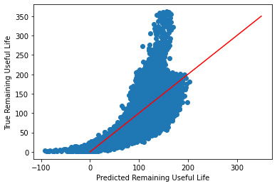
This plot shows a clear curve in the data which suggests we may be able to transform the data to get better performance. Let's try taking the log of the RUL to fix this.

log_y_train = np.log(y_train)
log_y_validate = np.log(y_validate)
reg.fit(X_train, log_y_train)
y_hat = reg.predict(X_validate)
#log_y_train.isna().sum()

print('Training Cross Validation Score: ', cross_val_score(reg, X_train, y_train, cv=5))
print('Validation Cross Validation Score: ', cross_val_score(reg, X_validate, log_y_validate, cv=5))
print('Validation R^2: ', r2_score(log_y_validate, y_hat))
print('Validation MSE: ', mean_squared_error(log_y_validate, y_hat))

Training Cross Validation Score:  [0.69888362 0.54057989 0.63081576 0.55132441 0.51100305]
Validation Cross Validation Score:  [0.67334079 0.72128858 0.65043858 0.71438363 0.56484904]
Validation R^2:  0.6915045493347627
Validation MSE:  0.2984384342830433

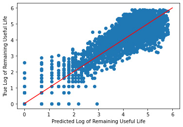
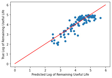
_ = plt.scatter(y_hat, log_y_validate)
_ = plt.plot([0, 6], [0, 6], "r")
_ = plt.xlabel("Predicted Log of Remaining Useful Life")
_ = plt.ylabel("True Log of Remaining Useful Life")

As you can tell, after the transformation of the data, we got a much more reasonable plot along the diagonal.

Decision Tree Regressor

Let's try another model to see if it performs better.

Decision trees are predictive models that use a set of binary rules to calculate a target value. A decision tree is arriving at an estimate by asking a series of questions to the data, each question narrowing our possible values until the model get confident enough to make a single prediction. Here's a visual example of a decision tree regressor from https://gdcoder.com/decision-tree-regressor-explained-in-depth/

Fitting the model

# trying decision tree regressor
from sklearn.tree import DecisionTreeRegressor

dt_reg = DecisionTreeRegressor()
dt_reg.fit(X_train, y_train)
y_hat = dt_reg.predict(X_validate)

Assessing Performance

print('Training Cross Validation Score: ', cross_val_score(dt_reg, X_train, y_train, cv=5))
print('Validation Cross Validation Score: ', cross_val_score(dt_reg, X_validate, y_validate, cv=5))
print('Validation R^2: ', r2_score(y_validate, y_hat))
print('Validation MSE: ', mean_squared_error(y_validate, y_hat))

Training Cross Validation Score:  [0.35184965 0.06401961 0.26987918 0.24646428 0.34449397]
Validation Cross Validation Score:  [ 0.34478644  0.36825102  0.08006531  0.20222369 -1.89180928]
Validation R^2:  0.14566532645905728
Validation MSE:  4334.829166666666

Plotting Predicted vs True Values

_ = plt.scatter(y_hat, y_validate)
_ = plt.plot([0, 350], [0, 350], "r")
_ = plt.xlabel("Predicted Remaining Useful Life")
_ = plt.ylabel("True Remaining Useful Life")

While this plot is symmetric, after 50 or so cycles it it's performance drastically decreases. Let's try using the transformed data like we did with linear regression.

dt_reg.fit(X_train, log_y_train)
y_hat = dt_reg.predict(X_validate)
print('Training Cross Validation Score: ', cross_val_score(dt_reg, X_train, log_y_train, cv=5))
print('Validation Cross Validation Score: ', cross_val_score(dt_reg, X_validate, log_y_validate, cv=5))
print('Validation R^2: ', r2_score(log_y_validate, y_hat))
print('Validation MSE: ', mean_squared_error(log_y_validate, y_hat))
_ = plt.scatter(y_hat, log_y_validate)
_ = plt.plot([0, 6], [0, 6], "r")
_ = plt.xlabel("Predicted Log of Remaining Useful Life")
_ = plt.ylabel("True Log of Remaining Useful Life")

Training Cross Validation Score:  [0.77002853 0.70817928 0.75497914 0.68358901 0.69388449]
Validation Cross Validation Score:  [0.66017649 0.72371054 0.53224588 0.70034248 0.50563546]
Validation R^2:  0.6542589454556127
Validation MSE:  0.3344698236654492

While the model does better with the transformed data, Linear Regression still has better performance.

K-Nearest Neighbors Regressor

Let's try one last model to see if it performs better.

Regression with K-Nearest Neighbors takes a y-value, then looks at the data and averages all the X points that are closest to that y-value. This average is the prediction. A visual of this from https://towardsdatascience.com/the-basics-knn-for-classification-and-regression-c1e8a6c955:

The blue points are the given data, the blue points circled in red are the nearest neighbors of the Y value, represented by the vertical red lines. The predictions, which are averages of the blue points circled in red, are the red dots on the lines.

Fitting the Model

from sklearn.neighbors import KNeighborsRegressor

kn_reg = DecisionTreeRegressor()
kn_reg.fit(X_train, y_train)
y_hat = kn_reg.predict(X_validate)

Assessing Performance

print('Training Cross Validation Score: ', cross_val_score(kn_reg, X_train, y_train, cv=5))
print('Validation Cross Validation Score: ', cross_val_score(kn_reg, X_validate, y_validate, cv=5))
print('Validation R^2: ', r2_score(y_validate, y_hat))
print('Validation MSE: ', mean_squared_error(y_validate, y_hat))

Training Cross Validation Score:  [0.35758267 0.0736068  0.25672278 0.23704877 0.32959209]
Validation Cross Validation Score:  [ 0.3644445   0.3667751   0.10499852  0.22457352 -1.93173184]
Validation R^2:  0.14180190709216056
Validation MSE:  4354.431862745098

Plotting Predicted vs True Values

_ = plt.scatter(y_hat, y_validate)
_ = plt.plot([0, 350], [0, 350], "r")
_ = plt.xlabel("Predicted Remaining Useful Life")
_ = plt.ylabel("True Remaining Useful Life")

While this plot is symmetric, after 50 or so cycles it it's performance drastically decreases. Let's try using the transformed data like we did with linear regression.

kn_reg.fit(X_train, log_y_train)
y_hat = kn_reg.predict(X_validate)
print('Training Cross Validation Score: ', cross_val_score(dt_reg, X_train, log_y_train, cv=5))
print('Validation Cross Validation Score: ', cross_val_score(dt_reg, X_validate, log_y_validate, cv=5))
print('Validation R^2: ', r2_score(log_y_validate, y_hat))
print('Validation MSE: ', mean_squared_error(log_y_validate, y_hat))
_ = plt.scatter(y_hat, log_y_validate)
_ = plt.plot([0, 6], [0, 6], "r")
_ = plt.xlabel("Predicted Log of Remaining Useful Life")
_ = plt.ylabel("True Log of Remaining Useful Life")

Training Cross Validation Score:  [0.77136845 0.7052402  0.75711344 0.6900989  0.69191554]
Validation Cross Validation Score:  [0.66254355 0.72646867 0.51679784 0.69416712 0.50404909]
Validation R^2:  0.655829127904749
Validation MSE:  0.33295082949341687

Trying Our Model On Test Data

Now that we've used the training data to find the best model, it's time to test our model on the test data! Remember, from the documentation we read in at the beginning, "In the test set, the time series ends some time prior to system failure." Let's take a look at the test data to see what we have..

test.head()

We also have the correct outputs saved in RUL, but if you remember, our best model was fit on the log(y), so we need to transform the correct RUL outputs in order to correctly compare our predictions with the true remaining useful life.

# taking log of y values
y_test = np.log(RUL)

#test_grp = train["cycle"].groupby(test["unit"])
#test_rul_lst = [j for i in test["unit"].unique() for j in np.array(test_grp.get_group(i)[::-1])]

Using our model to predict RUL for test data

Earlier, when we trained the PCA on the training data, we transformed the test data with it and saved it as test_df which is the dataframe we will use as our input, X.

# Test Data with PCA (fit on training data) applied 
test_df.head()

Now, we use the model we trained above on the training data to predict the remaining useful life of the test data.

# predict remaining useful life
y_hat_test = reg.predict(test_df)

#make predictions into a dataframe
y_hat_test = pd.DataFrame(y_hat_test)

# add unit column back in so that we know which predictions go with which unit
y_hat_test.insert(0, "unit", test["unit"])

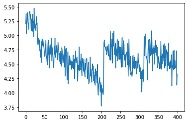
Since our model actually makes a prediction for each row of data, we can plot our predictions and see if the remaining useful life plot looks like it is changing for each unit. By plotting the first 400 predictions for each row, it is clear that out model is correctly predicting that for each unit, the remaining useful life is decreasing over time.

_ = plt.plot(y_hat_test[0][0:400])

Ultimately, we want a prediction output of one value for each unit that tell us the remaining useful life for each unit in the data. Right now, we have one prediction per row of data, and each unit has many rows. To get just one prediction per unit, we will loop through y_hat_test dataframe of the predictions, and grab the last prediction for each unit since that will tell us the final number of cycles for the remaining useful life..

rul_pred = []

# loop through all units
for each in range(1,101):
    # get data for one unit at a time
    unit_data = y_hat_test[y_hat_test["unit"] == each]
    
    # get last prediction for that unit and add it to the list of predictions
    rul_pred.append(unit_data.tail(1).iloc[0][0])
rul_pred = pd.DataFrame(rul_pred)

rul_pred.head()

print('Training Cross Validation Score: ', cross_val_score(reg, rul_pred, y_test, cv=5))
print('Validation Cross Validation Score: ', cross_val_score(reg, rul_pred, y_test, cv=5))
print('Validation R^2: ', r2_score(y_test, rul_pred))
print('Validation MSE: ', mean_squared_error(y_test, rul_pred))

Training Cross Validation Score:  [0.47738765 0.81889428 0.65937406 0.81015806 0.80221537]
Validation Cross Validation Score:  [0.47738765 0.81889428 0.65937406 0.81015806 0.80221537]
Validation R^2:  0.7565921223696981
Validation MSE:  0.1702170255729099

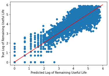
_ = plt.scatter(rul_pred, y_test)
_ = plt.plot([0, 6], [0, 6], "r")
_ = plt.xlabel("Predicted Log of Remaining Useful Life")
_ = plt.ylabel("True Log of Remaining Useful Life")

Conclusion

In this tutorial, we wanted to be able to predict a machine's remaining useful life given sensor measurements and operational settings over time in cycles. To do this, we read in the data, processed it, split it into training, validation, and test sets, applied dimensionality reduction, and finally ran three different models on the training and validation data. Then, we looked to the model accuracy metrics to decide on a model to move forward with for predictions. When looking at r-squared, linear regression was the best model with an r-squared of 71% compared to 68% for the other two models. When applying our model to the test data, we get an r-squared of 74% which is slightly better performance than it was on the training set. Now you can go forward knowing how many cycle's are left in this simulated engine's life!

Next Steps

Possible next steps to improve model performance:

• research other regression models and try implementing them
• try tuning parameters in sklearn's models that we used above
• try different implementations of PCA (we got # of features to explain 95% of the variance in the data. Maybe try changing this to a higher or lower percentage)
• research the models others have made on this dataset and try implementing them for yourself