
Suggest a Dataset
![]()
import pandas as pd
import matplotlib.pyplot as plt
import numpy as np
import statsmodels.formula.api as smf

from pandas.plotting import scatter_matrix

from sklearn import datasets, linear_model
from sklearn.metrics import mean_squared_error, r2_score
from sklearn.linear_model import LinearRegression
from sklearn.metrics import mean_absolute_error
from sklearn.model_selection import train_test_split
from sklearn.tree import DecisionTreeRegressor
from sklearn.ensemble import RandomForestRegressor
#df = pd.read_excel('dataset.xlsx')
df = pd.read_excel('powerplant.xlsx')
from IPython.display import Image
Image(filename='powerplantphoto.jpg',width=450, height=450)

The dataset used contains 9568 data points collected from a Combined Cycle Power Plant over 6 years (2006-2011), when the power plant was set to work with full load. Features consist of hourly average ambient variables Temperature (T), Ambient Pressure (AP), Relative Humidity (RH) and Exhaust Vacuum (V) to predict the net hourly electrical energy output (EP) of the plant. A combined cycle power plant (CCPP) is composed of gas turbines (GT), steam turbines (ST) and heat recovery steam generators. In a CCPP, the electricity is generated by gas and steam turbines, which are combined in one cycle, and is transferred from one turbine to another. While the Vacuum is colected from and has effect on the Steam Turbine, he other three of the ambient variables effect the GT performance
The following table shows what the dataset looks like
df.head()
| AT | V | AP | RH | PE | |
|---|---|---|---|---|---|
| 0 | 14.96 | 41.76 | 1024.07 | 73.17 | 463.26 |
| 1 | 25.18 | 62.96 | 1020.04 | 59.08 | 444.37 |
| 2 | 5.11 | 39.40 | 1012.16 | 92.14 | 488.56 |
| 3 | 20.86 | 57.32 | 1010.24 | 76.64 | 446.48 |
| 4 | 10.82 | 37.50 | 1009.23 | 96.62 | 473.90 |
df.describe()
| AT | V | AP | RH | PE | |
|---|---|---|---|---|---|
| count | 9568.000000 | 9568.000000 | 9568.000000 | 9568.000000 | 9568.000000 |
| mean | 19.651231 | 54.305804 | 1013.259078 | 73.308978 | 454.365009 |
| std | 7.452473 | 12.707893 | 5.938784 | 14.600269 | 17.066995 |
| min | 1.810000 | 25.360000 | 992.890000 | 25.560000 | 420.260000 |
| 25% | 13.510000 | 41.740000 | 1009.100000 | 63.327500 | 439.750000 |
| 50% | 20.345000 | 52.080000 | 1012.940000 | 74.975000 | 451.550000 |
| 75% | 25.720000 | 66.540000 | 1017.260000 | 84.830000 | 468.430000 |
| max | 37.110000 | 81.560000 | 1033.300000 | 100.160000 | 495.760000 |
Features consist of hourly average ambient variables
| Variables | ||||
|---|---|---|---|---|
| Temperature (T) | in the range 1.81°C and 37.11°C | |||
| Ambient Pressure (AP) | in the range 992.89-1033.30 milibar | |||
| Relative Humidity (RH) | in the range 25.56% to 100.16% | |||
| Exhaust Vacuum (V) | in the range 25.36-81.56 cm Hg | |||
| Net hourly electrical energy output (EP) | 420.26-495.76 MW |
Before using the dataset, we must make sure that there are no null entries in the data set which may cause errors later on. As seen below, all the parameters in the data set are non-null
df.info()
<class 'pandas.core.frame.DataFrame'>
RangeIndex: 9568 entries, 0 to 9567
Data columns (total 5 columns):
 #   Column  Non-Null Count  Dtype
---  ------  --------------  -----
 0   AT      9568 non-null   float64
 1   V       9568 non-null   float64
 2   AP      9568 non-null   float64
 3   RH      9568 non-null   float64
 4   PE      9568 non-null   float64
dtypes: float64(5)
memory usage: 373.9 KB
scatter_matrix(df, figsize=(14, 14),diagonal="kde");
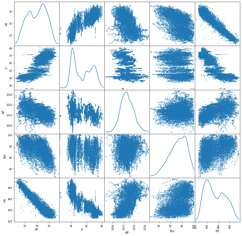
From these scatter plots, temperature shows the strongest linear relationship with the hourly electrical energy output. Exhaust vacuum appears to have a linear relationship, though at a lesser extent.
On the other hand, the Ambient Pressure seems to have a weak linear correlation with the output whereas relative humidity appears to have little to no impact on the output.
The initial observation of the data suggests that we will need to use a linear regression model to predict the power output. We will put that finding to a test.
Using the statsmodels library, we obtain the following relationship between variables and the output (PE):
lm = smf.ols(formula="PE ~ AT + V + AP + RH", data=df).fit()
lm.params
Intercept    454.609274
AT            -1.977513
V             -0.233916
AP             0.062083
RH            -0.158054
dtype: float64
The above values tell us that we can use the following formula to predict the output power using AT, V, AP, and RH:
PE = 454.609274 - 1.977513 * AT - 0.233916 * V + 0.062083 * AP - 0.158054 * RHTo test if the model is able to predict the output, we will use the first entry of the data set:
lm.predict(pd.DataFrame({"AT": [8.34], "V": [40.77], "AP": [1010.84], "RH": [90.01]}))
0    477.109516
dtype: float64
The actual observed value is 480.48, which is not very far from the predicted value from the formula derived above.
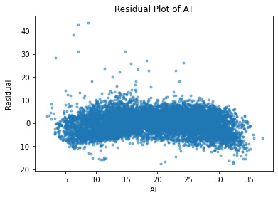
A residual plot is a graph that shows the residuals on the y-axis and the independent variable on the x-axis. If the points in a residual plot are randomly dispersed around the x-axis, a linear regression model is appropriate for the data.
I will plot a residual plot for each indenpendent variable to further explore if a linear regression model is a good model for our prediction.
residuals = lm.predict(df) - df.PE
plt.plot(df.AT, residuals, ".", alpha=0.5)
plt.xlabel("AT")
plt.ylabel("Residual");
plt.title("Residual Plot of AT")
Text(0.5, 1.0, 'Residual Plot of AT')
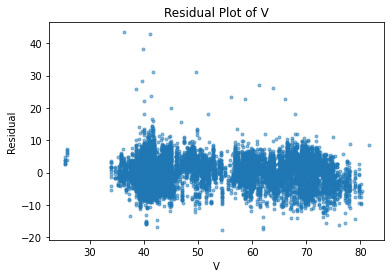
plt.plot(df.V, residuals, ".", alpha=0.5)
plt.xlabel("V")
plt.ylabel("Residual");
plt.title("Residual Plot of V")
Text(0.5, 1.0, 'Residual Plot of V')
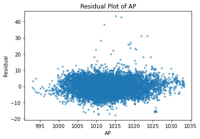
plt.plot(df.AP, residuals, ".", alpha=0.5)
plt.xlabel("AP")
plt.ylabel("Residual");
plt.title("Residual Plot of AP")
Text(0.5, 1.0, 'Residual Plot of AP')
plt.plot(df.RH, residuals, ".", alpha=0.5)
plt.xlabel("RH")
plt.ylabel("Residual");
plt.title("Residual Plot of RH")
Text(0.5, 1.0, 'Residual Plot of RH')
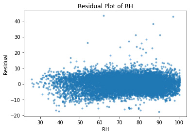
As expected, all of the independent variables in the data set are showing a random pattern. Some residuals are negative while others are positive; there is no non-random shapes such as U-shaped or inverted U. We can conclude at this point that for our predictions, linear regression is a good candidate.
We have established that the independent variables in the data set can be used for linear regression to make predictions of the dependent variable, PE (output). Now, we will test different models to make the prediction more accurate. Though we have obtained a linear model earlier using the statsmodel library, it was a simple and rudimentary mathematical derivation using the data.
This time, we will take a more elaborate approach to make the prediction.
We will use the sklearn library, which provides different machine learning models.
For the different models that are used in this article, each model will divde the dataset into two subsets, the train dataset and the test dataset, in a 80-20 split.
The train dataset is a subset to train a model using a type of machine learning technique, and the test dataset is a subset to test the trained model.
First, we will use the linear regression algorithm to predict the dataset.
We will use four predictors, as listed below, to train. The first model uses only the 'AP', the second model uses 'AT' and 'V', the third model 'AT', 'V', 'AP', and the fourth and final model will use all the independent variables in the dataset.
Using different predictors will show which of the features are most useful in predicting the output.
One of the most important steps in creating a machine learning model is to divide the data set into good predictors to train the algorithm on.
For this project, I have created four predictors.
The first one, df_1, uses just the 'AT' variable because the temperature showed the highest linearity with the output. The second predictor, df_2, contains 'AT' and 'V', the two variables that had the most linear relationship with the output. The third set, df_3, has 'AT', 'V', and 'AP' variables, and the fourth set, df_4, has all of the independent variables in the data set.
df_1 = df['AT']
df_2 = df[['AT', 'V']]
df_3 = df[['AT', 'V', 'AP']]
df_4 = df[['AT', 'V', 'AP', 'RH']]

y = df['PE']
Linear regression model is based on supervised learning, where independent variables are valued based on the dependent varaible (the output). As the name suggests, the model finds a linear relationship between the independent variables and the dependent variable.
The following figures shows what the linear regression model looks like:
 ```python Image(filename='linearregression.png',width=600, height=600) ```
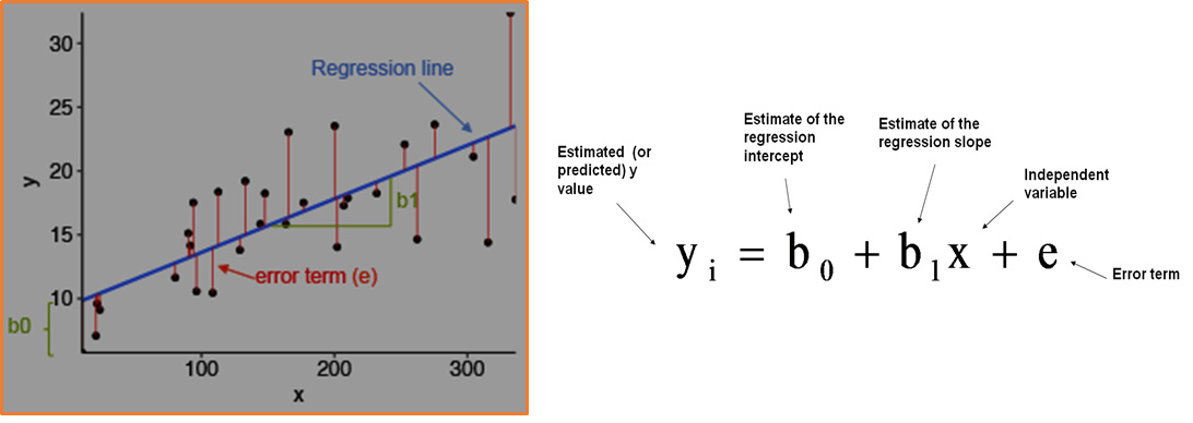
We will first use the Linear Regression Model from the sklearn library to train our machine learning model.
We will obtain the Root Mean Squared Error (RMSE), R-Squared, and Mean Absolute Error values for each predictor set.
Here are the brief explanation for each value:
Root Mean Squared Error (RMSE): measures the average error performed by the model in predicting the outcome for an observation.R-Squared: It means how much of the variation in the target variable that can be explained by the set of features used in training the model.Mean Absolute Error: measures how far predicted values are away from the actual values.To put these definitions in layman's terms, the lower values of RMSE and MAE and the higher value of R-squared score mean better predictors of the output.
I will now run the linear regression algorithm on all four sets of the predictors and obtain the root mean squared error, r-squared, and mean absolute values:
X_train, X_test, y_train, y_test = train_test_split(df_1, y, test_size = 0.2, random_state = 0)

# Linear Regression with one parameter
regressor = LinearRegression()
regressor.fit(X_train.values.reshape(-1,1), y_train.values.reshape(-1,1))

y_pred = regressor.predict(X_test.values.reshape(-1,1))

mse = mean_squared_error(y_test, y_pred)
rmse = np.sqrt(mse)
print('rmse: ', rmse)

r_squared = r2_score(y_test, y_pred)
print('r_squared: ', r_squared)

mae = mean_absolute_error(y_test, y_pred)
print('mae: ', mae)
rmse:  5.272562059337881
r_squared:  0.9049536175690114
mae:  4.174438156494201
X_train, X_test, y_train, y_test = train_test_split(df_2, y, test_size = 0.2, random_state = 0)

# Linear Regression with two parameters
regressor = LinearRegression()
regressor.fit(X_train, y_train)

y_pred = regressor.predict(X_test)

mse = mean_squared_error(y_test, y_pred)
rmse = np.sqrt(mse)
print('rmse: ', rmse)

r_squared = r2_score(y_test, y_pred)
print('r_squared: ', r_squared)

mae = mean_absolute_error(y_test, y_pred)
print('mae: ', mae)
rmse:  4.848681080539322
r_squared:  0.9196215863801613
mae:  3.854553363596844
X_train, X_test, y_train, y_test = train_test_split(df_3, y, test_size = 0.2, random_state = 0)

# Linear Regression with 3 parameters
regressor = LinearRegression()
regressor.fit(X_train, y_train)

y_pred = regressor.predict(X_test)

mse = mean_squared_error(y_test, y_pred)
rmse = np.sqrt(mse)
print('rmse: ', rmse)

r_squared = r2_score(y_test, y_pred)
print('r_squared: ', r_squared)

mae = mean_absolute_error(y_test, y_pred)
print('mae: ', mae)
rmse:  4.782396128432508
r_squared:  0.9218042258408323
mae:  3.8234137990557127
X_train, X_test, y_train, y_test = train_test_split(df_4, y, test_size = 0.2, random_state = 0)

# Linear Regression with 4 parameters
regressor = LinearRegression()
regressor.fit(X_train, y_train)

y_pred = regressor.predict(X_test)

mse = mean_squared_error(y_test, y_pred)
rmse = np.sqrt(mse)
print('rmse: ', rmse)

r_squared = r2_score(y_test, y_pred)
print('r_squared: ', r_squared)

mae = mean_absolute_error(y_test, y_pred)
print('mae: ', mae)
rmse:  4.442262858442491
r_squared:  0.9325315554761302
mae:  3.566564655203823
The following table has all the RMSE, R_Squared, and MAE values for Linear Regression Model:
| df_1 | df_2 | df_3 | df_4 | |
|---|---|---|---|---|
| RMSE | 5.3324 | 4.848 | 4.78 | 4.44 |
| R2 | .9006 | .919 | .933 | .880 |
| MAE | 4.24 | 3.85 | 3.82 | 3.567 |
According to the table above, df_4, the set of predictors that contains all of the variables in the data set, gave the best predictions. df_2, with AT and V variables, which showed linearities with the output, was still not as good as df_3 or df_4. While the two variables, AP and RH, seem to have little linear relationship with the output, they are still useful in predicting the output in combination with the other variables.
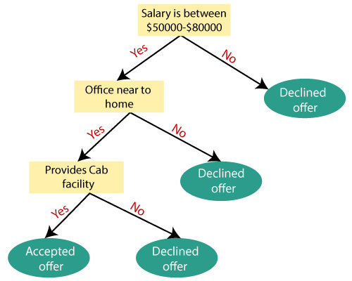
The next technique we will use is the decision tree regression. As the name suggests, this technique involves using a tree structure. The dataset is broken down into smaller and smaller subsets while an associated decision tree is incrementally developed.
The tree starts from a root node, and branches out with interior nodes until leaf nodes are created at the end. Each interior node asks a True/False question, and the leaf nodes represent the predicted outcome.
The following shows an example of a decision tree regression:
Image(filename='decisiontreemodel.png',width=450, height=450)
# Decision Tree Regression with 1 parameters

X_train, X_test, y_train, y_test = train_test_split(df_1, y, test_size = 0.2, random_state = 0)

dt_regressor= DecisionTreeRegressor()
dt_regressor.fit(X_train.values.reshape(-1,1), y_train.values.reshape(-1,1))

y_pred = dt_regressor.predict(X_test.values.reshape(-1,1))

mse = mean_squared_error(y_test, y_pred)
rmse = np.sqrt(mse)
print('rmse: ', rmse)

r_squared = r2_score(y_test, y_pred)
print('r_squared: ', r_squared)

mae = mean_absolute_error(y_test, y_pred)
print('mae: ', mae)
rmse:  5.93651805220736
r_squared:  0.8795086758953446
mae:  4.633473127113801
# Decision Tree Regression with 2 parameters

X_train, X_test, y_train, y_test = train_test_split(df_2, y, test_size = 0.2, random_state = 0)

dt_regressor= DecisionTreeRegressor()
dt_regressor.fit(X_train, y_train)

y_pred = dt_regressor.predict(X_test)

mse = mean_squared_error(y_test, y_pred)
rmse = np.sqrt(mse)
print('rmse: ', rmse)

r_squared = r2_score(y_test, y_pred)
print('r_squared: ', r_squared)

mae = mean_absolute_error(y_test, y_pred)
print('mae: ', mae)
rmse:  4.602614244946659
r_squared:  0.9275728583672498
mae:  3.1918382096830378
# Decision Tree Regression with 3 parameters

X_train, X_test, y_train, y_test = train_test_split(df_3, y, test_size = 0.2, random_state = 0)

dt_regressor= DecisionTreeRegressor()
dt_regressor.fit(X_train, y_train)

y_pred = dt_regressor.predict(X_test)

mse = mean_squared_error(y_test, y_pred)
rmse = np.sqrt(mse)
print('rmse: ', rmse)

r_squared = r2_score(y_test, y_pred)
print('r_squared: ', r_squared)

mae = mean_absolute_error(y_test, y_pred)
print('mae: ', mae)
rmse:  4.39425968826849
r_squared:  0.9339818075689313
mae:  3.061844305120167
# Decision Tree Regression with 4 parameters

X_train, X_test, y_train, y_test = train_test_split(df_4, y, test_size = 0.2, random_state = 0)

dt_regressor= DecisionTreeRegressor()
dt_regressor.fit(X_train, y_train)

y_pred = dt_regressor.predict(X_test)

mse = mean_squared_error(y_test, y_pred)
rmse = np.sqrt(mse)
print('rmse: ', rmse)

r_squared = r2_score(y_test, y_pred)
print('r_squared: ', r_squared)

mae = mean_absolute_error(y_test, y_pred)
print('mae: ', mae)
rmse:  4.87158453620759
r_squared:  0.9188604344770246
mae:  3.1281765935214207
The following table has all the RMSE, R_Squared, and MAE values for the Decision Tree Regression Model:
| df_1 | df_2 | df_3 | df_4 | |
|---|---|---|---|---|
| RMSE | 5.8581 | 4.66 | 4.399 | 4.78 |
| R2 | .880 | .926 | .934 | .922 |
| MAE | 3.543 | 3.228 | 3.06 | 3.12 |
df_3, the set of predictors with the variables AT, V, AP, gave the best predictions among the four sets.
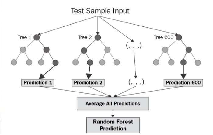
Finally, the random forest regression model is used.
Random forest is an ensemble of decision trees. In other words, many trees are constructed in "random" way to form a Random Forest, and the trees formed in the forest are averaged to produce a prediction. As a result, this method gives a better result than having just one tree.
Image(filename='randomforestregression.png',width=450, height=450)
# Random Forest Regression with 1 parameter
X_train, X_test, y_train, y_test = train_test_split(df_1, y, test_size = 0.2, random_state = 0)

rf_regressor= RandomForestRegressor()
rf_regressor.fit(X_train.values.reshape(-1,1), y_train.values.reshape(-1,1))

y_pred = rf_regressor.predict(X_test.values.reshape(-1,1))


mse = mean_squared_error(y_test, y_pred)
rmse = np.sqrt(mse)
print('rmse: ', rmse)

r_squared = r2_score(y_test, y_pred)
print('r_squared: ', r_squared)

mae = mean_absolute_error(y_test, y_pred)
print('mae: ', mae)
# Random Forest Regression with 2 parameters
X_train, X_test, y_train, y_test = train_test_split(df_2, y, test_size = 0.2, random_state = 0)

rf_regressor= RandomForestRegressor()
rf_regressor.fit(X_train, y_train)

y_pred = rf_regressor.predict(X_test)


mse = mean_squared_error(y_test, y_pred)
rmse = np.sqrt(mse)
print('rmse: ', rmse)

r_squared = r2_score(y_test, y_pred)
print('r_squared: ', r_squared)

mae = mean_absolute_error(y_test, y_pred)
print('mae: ', mae)
# Random Forest Regression with 3 parameters
X_train, X_test, y_train, y_test = train_test_split(df_3, y, test_size = 0.2, random_state = 0)

rf_regressor= RandomForestRegressor()
rf_regressor.fit(X_train, y_train)

y_pred = rf_regressor.predict(X_test)


mse = mean_squared_error(y_test, y_pred)
rmse = np.sqrt(mse)
print('rmse: ', rmse)

r_squared = r2_score(y_test, y_pred)
print('r_squared: ', r_squared)

mae = mean_absolute_error(y_test, y_pred)
print('mae: ', mae)
# Random Forest Regression with 4 parameters
X_train, X_test, y_train, y_test = train_test_split(df_4, y, test_size = 0.2, random_state = 0)

rf_regressor= RandomForestRegressor()
rf_regressor.fit(X_train, y_train)

y_pred = rf_regressor.predict(X_test)


mse = mean_squared_error(y_test, y_pred)
rmse = np.sqrt(mse)
print('rmse: ', rmse)

r_squared = r2_score(y_test, y_pred)
print('r_squared: ', r_squared)

mae = mean_absolute_error(y_test, y_pred)
print('mae: ', mae)
The following table has all the RMSE, R_Squared, and MAE values for the Random Forest Regression Model:
| df_1 | df_2 | df_3 | df_4 | |
|---|---|---|---|---|
| RMSE | 5.677 | 3.501 | 3.273 | 3.203 |
| R2 | .889 | .9579 | .963 | .965 |
| MAE | 4.4365 | 2.6216 | 2.39 | 2.35 |
The df_2 predictor gave the best result out of the four sets. This
The following table shows all of the results from the three machine learning models:
| LR | LR | LR | LR | DTR | DTR | DTR | DTR | RFR | RFR | RFR | RFR | |
|---|---|---|---|---|---|---|---|---|---|---|---|---|
| df_1 | df_2 | df_3 | df_4 | df_1 | df_2 | df_3 | df_4 | df_1 | df_2 | df_3 | df_4 | |
| RMSE | 5.3324 | 4.848 | 4.78 | 4.44 | 5.8581 | 4.66 | 4.399 | 4.78 | 5.677 | 3.501 | 3.273 | 3.203 |
| R2 | .9006 | .919 | .922 | .933 | .880 | .926 | .934 | .922 | .889 | .9579 | .963 | .965 |
| MAE | 4.24 | 3.85 | 3.82 | 3.567 | 3.543 | 3.228 | 3.06 | 3.12 | 4.4365 | 2.6216 | 2.39 | 2.35 |
The random forest regression model gave the most accurate predictions out of the three models, followed by the decision tree regression model, and the linear regression model.
In case of predictions, random forest model provides the best result because random forest model complements the disadvantages of the decision tree model. We have briefly touched on how the decision tree model works. It is a series of if/else questions to get the most optimal result. The main problem of this method is overfitting, which is the production of an analysis that corresponds too closely or exactly to a particular set of data, and may therefore fail to fit additional data or predict future obeservations reliably. In other words, to get the most optimal result using the decision tree model, choosing the if/else questions is critical. However, there are so many variations that each node can produce, and in the end, we will be left with less than ideal predictions.
Random forest model mitigates the issue by creating an ensemble of decision trees to make predictions. The overfitting problem of the decision tree model is eliminated by learning on a random sample, and at each node, a random set of features are considered for splitting. Both mechanisms create diversity among the trees.
Lastly, the linear regression model performed most poorly out of the tree because in a real life model, especially with many variables, we cannot expect the outcome to be completely linear with the independent varaibles.
Suggest a Dataset